Fastest Zero Values Filter In / Out

Fastest way to filter rows for zero values:

  • Format the column in accounting format (Alt+H N A in recent versions of Excel)
  • Autofilter
  • To keep only zero values, type in the search bar, then OK
  • To filter out zero values, type . in the search bar, then OK

This works because in accounting format, negative numbers are represented by parentheses, and zero values are represented as a dash.

COUNTIFS Assistant – COUNTIFSRANGE Custom function

I was tired of manually creating long COUNTIFS formulas to identify duplicates in a dataset, so I created the following user-defined function.

The first parameter is the range you’re counting values in.

The second parameter is the range containing the values sought for.

As an example, using the formula
=COUNTIFSRANGE($A$2:$H$4968,A2:H2)
is the equivalent of writing out the following extended COUNTIFS:
=COUNTIFS($A$2:$A$4968,$A$2,$B$2:$B$4968,$B$2,$C$2:$C$4968,$C$2,$D$2:$D$4968,$D$2,$E$2:$E$4968,$E$2,$F$2:$F$4968,$F$2,$G$2:$G$4968,$G$2,$H$2:$H$4968,$H$2)
Public Function COUNTIFSRANGE(rgData As Range, rgValues As Range) As Long

Dim lColLoop As Long, sFormula
If rgData.Columns.Count <> rgValues.Columns.Count Or rgValues.Rows.Count > 1 Then
COUNTIFSRANGE = “#N/A”
Else

For lColLoop = 1 To rgData.Columns.Count
sFormula = sFormula & “,” & rgData.Columns(lColLoop).Address & “,” & rgValues.Columns(lColLoop).Address
Next

COUNTIFSRANGE = Evaluate(“=COUNTIFS(” & Mid(sFormula, 2) & “)”)

Debug.Print “=COUNTIFS(” & Mid(sFormula, 2) & “)”

End If


End Function
Thomas

Retrieve all comments in a workbook

Hello all,

You want to retrieve all the comments from a workbook in a neat way, without having to print the workbook (you know you can print the comments in a separate page, right?). The following sub will pull all comments and put them in a new worksheet, neatly, with the sheet title, hyperlinked cell reference, the cell value and the cell comment.

Try it, you might like it.

Sub RetrieveCasdfomments()
‘get all comments from a workbook and put them in a new worksheet
Dim rgCmt As Range, rgComments As Range, lRowLoop As Long, shtLoop As Worksheet, shtComments As Worksheet

Application.ScreenUpdating = False
Application.Calculation = xlCalculationManual

Sheets.Add before:=Sheets(1)
Set shtComments = ActiveSheet

With shtComments

‘create and format the comment summary sheet
shtComments.Name = “Comments”

With .Columns(“A:D”)

.VerticalAlignment = xlTop
.WrapText = True

End With

.Columns(“C”).ColumnWidth = 15
.Columns(“D”).ColumnWidth = 60
.PageSetup.PrintGridlines = True

.[a1] = “Sheet”
.[b1] = “Cell”
.[c1] = “Value”
.[d1] = “Comment”

.Rows(1).Font.Bold = True

.Tab.Color = 255
.Tab.TintAndShade = 0

End With

lRowLoop = 2

For Each shtLoop In ActiveWorkbook.Worksheets

‘loop through all worksheets and retrieve the comments
If shtLoop.Name <> shtComments.Name And shtLoop.Comments.Count > 0 Then

On Error Resume Next
Set rgComments = shtLoop.Cells.SpecialCells(xlCellTypeComments)

If Err = 0 Then

For Each rgCmt In rgComments.Cells

If Trim(rgCmt.Comment.Text) <> “” Then

shtComments.Cells(lRowLoop, 1) = shtLoop.Name
shtComments.Hyperlinks.Add Anchor:=shtComments.Cells(lRowLoop, 2), Address:=””, _
SubAddress:=”‘” & shtLoop.Name & “‘!” & rgCmt.Address(0, 0), TextToDisplay:=rgCmt.Address(0, 0)
shtComments.Cells(lRowLoop, 3) = “‘” & rgCmt.Text
shtComments.Cells(lRowLoop, 4) = “‘” & rgCmt.Comment.Text
lRowLoop = lRowLoop + 1

End If

Next rgCmt

Else

Err.Clear

End If

End If

Next shtLoop

shtComments.Activate

‘clean up
If Application.WorksheetFunction.CountA(shtComments.Columns(1)) = 1 Then

MsgBox “No comments in workbook”
Application.DisplayAlerts = False
shtComments.Delete
Application.DisplayAlerts = True

End If

Application.Calculation = xlCalculationAutomatic ‘xl95 uses xlAutomatic
Application.ScreenUpdating = True
End Sub

Thomas
How to start building a macro arsenal

Face it, macros will make your life easier. You might not know how to write them yet but it shouldn’t deter you from using them. This post will make it easy for you to start collecting macros and keeping them handy for when the need strikes.

First, you will need a personal macro workbook. Macros are stored in workbooks and I’ll give you three types of workbooks:

  • The plain old workbook
  • The personal macro workbook
  • The add-in, which enables easy distribution of macros and functions. I won’t get into any more details on the add-ins here.

You should only store in the workbook macros that are either only relevant to that specific workbook, or are triggered by specific events on the workbook, or that need to accompany the workbook if you were to send it to somebody else.

All other macros should go to your personal macro workbook.

Do you have a personal macro workbook? If you don’t know the answer, it’s probably no, but I’ll show you how to set it up. The easiest way is to record a macro. A few options for this:

  • Use the shortcut Alt+t m r (for Tools \ Macro \ Record).
  • Click the Record Macro button on the Developer tab in the ribbon. It’s not installed by default, but you can right-click the ribbon, “Customize the Ribbon” and check the Developer box in the Main Tabs window to install it.
  • Right-click the status bar on the bottom left of your excel window (it should say Ready) and select Macro Recording, You now have a new status bar button to start (and stop) recording macros.

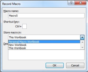
Once you’ve picked one of those options, you’ll see the following window:

Record Macro window

In the Store Macro In dropdown, select Personal Macro Workbook, then click OK. A small blue square (Stop Recording) will appear on the bottom left of your screen on the status bar. Click it (or use the same shortcut Alt+ t m r) to stop recording the macro.

You now have a personal macro workbook, stored somewhere in the depths of your user profile (something like C:\Users\UserName\AppData\Roaming\Microsoft\Excel\XLSTART depending on your version of windows). To see it, you’ll have to venture in the Visual Basic Editor, using the Alt+F11 shortcut, or press the Visual Basic button in the Developer tab of the Ribbon (see above). Expand the VBA Project (PERSONAL.XLSB), expand the Modules and you’ll see the first Module of your Personal Macro workbook, as shown in the screenshot below. Double-click to view the code, add any macros you want, and don’t forget to save.

Visual Basic Editor Screenshot

You can now close the Visual Basic Editor, your Personal Macro workbook should open whenever you open Excel and you can start filling it with wonderful macros!

Try it, you might like it.

Thomas

UPDATE: Once you have saved your macros, the easisest way to run them from Excel is to use the Alt+F8 shortcut, pick your macro and click OK.

Quick Summary for multi-tab workbooks

Hi all,

You inherited a workbook with multiple tabs, with all tabs containing the same structure. Maybe the tabs are split by region, or by month, or anything else. Of course, for proper analysis, you’ll want to consolidate all the tabs in one data tab, but this is not our goal right here.

Question: Assuming you need to keep the file in the current format, how can you quickly look at data from a specific cell in all the tabs at once.

Answer: Using the INDIRECT() function, which turns a string reference into a range you can use in formula.

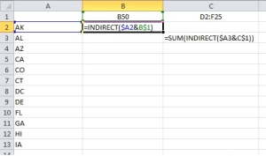
In a new sheet, build a table with your tab names in a column (you can also use my Table Of Contents macro), and the cell references in a row. Concatenate column and row to get a properly formed range reference, e.g. FL!A5, or ‘Northern Division’!B6:C20. Use the indirect function to return the reference in whatever formula you need. If you reference one cell, you can retrieve it directly. If you reference a range, you need to use it in a formula that accept ranges (SUM, COUNT, COUNTIF, etc.). If your tab name has special characters, such as a space, make sure you surround it with inverted commas.

In the screenshot below, the formulas are ready to be copied down, to pull cell B50 for each of your tabs, and the sum of range D2:F25 for each tab.

INDIRECT Function

INDIRECT Function example


Try it, you might like it.


Thomas


For more reading on the INDIRECT function, you can see the Microsoft Office website here.

Table Of Contents for multi-tab workbooks

Hi all,


A quick and dirty way to create a table of contents for a multi-tab excel workbook. Run the attached macro and it will create a new tab, with the list of all existing tabs and a hyperlink to each of them.

Try it, you might like it.

Sub IndexAllTabs()
‘creates table of contents for workbook
Dim sht As Worksheet, i As Long
Dim shtDone As Worksheet

Set shtDone = ActiveWorkbook.Sheets.Add

On Error Resume Next
shtDone.Name = “TOC”

If Err.Number <> 0 Then
    ActiveWorkbook.Sheets(“TOC”).Delete
    shtDone.Name = “TOC”
    Err.Clear
End If
i = 1

For Each sht In ActiveWorkbook.Sheets
    If sht.Name <> shtDone.Name Then
        shtDone.Hyperlinks.Add Anchor:=ActiveSheet.Cells(i, 1), Address:=””, SubAddress:= _
            “‘” & sht.Name & “‘!A1”, TextToDisplay:=sht.Name
        i = i + 1
    End If
Next

End Sub


Thomas

The Great Splitter And Sender Of Reports

On a monthly basis, at least, you’re faced with slew of reports that need to be sent to various managers, with some managers getting one part of the report, some getting others, and some getting all the parts.

You will usually have to copy tabs to new workbooks, save temporary files and e-mail them.

Here comes the Great Splitter And Sender of Reports to make your life easier and generally better: use the Command Center tab to define who gets which tabs in the workbook, set the parameters of the e-mail, etc. then press the Split and Send button to, you guessed it, split and send the tabs. You just have to go to Outlook to press Send on all those e-mails and you’re done.

To include that functionality to one of your report files, copy the Command Center tab and the module mSplitAndSend to your report workbook. Voilà.

Here’s the file: The Great Splitter and Sender of reports.

Try it, you might like it,

Thomas

Explode two lists with all values of the other

From time to time, and I must admit, it doesn’t happen often, but often enough to justify making a macro, you will want to match two lists, e.g. a list of employees and a list of G/L accounts, and get as a result a line for each possible combination of employees and accounts.

Image

Here’s the excel version.

1. Copy the code listed at the end of this post in a standard VB module

2. Select both ranges: you select the employee list with the mouse, then press Ctrl, release the mouse button (while still holding the Ctrl key down) and select the GL list.

3. Run the macro: you now have a new tab with the expanded list ready for consumption.

Try it, you might like it.

Thomas

Here’s the code:

Sub ExplodeLists()
Dim rg1 As range, rg2 As range, shtDest As Worksheet, rgCell As range
Dim lLoop As Long, lRowDest As Long

‘turn off updates to speed up code execution
With application
.ScreenUpdating = False
.EnableEvents = False
.Calculation = xlCalculationManual
End With

If selection.Areas.Count <> 2 Then
MsgBox “Select two areas to join”
Exit Sub
End If

Set rg1 = selection.Areas(1)
Set rg2 = selection.Areas(2)
Set shtDest = Worksheets.Add

lRowDest = 1

For lLoop = 1 To rg1.Rows.Count
shtDest.Cells(lRowDest, 1).Resize(rg2.Rows.Count, rg1.Columns.Count).Value = rg1.Rows(lLoop).Value
rg2.Copy shtDest.Cells(lRowDest, 1 + rg1.Columns.Count)
lRowDest = lRowDest + rg2.Rows.Count
Next

With application
.ScreenUpdating = True
.EnableEvents = True
.Calculation = xlCalculationAutomatic
End With

End Sub

Reports of all stripes with conditional formatting

Hi all,

Imagine you want alternating rows (or columns) in a report to have alternating colors. I don’t know, maybe you’re missing the days of tractor-feed paper.

One option is to convert your data in a table (Ctrl+T, or Insert \ Table). Other advantages come with the table like the ability to reference ranges in formulas with names instead of addresses, but the table doesn’t work in all cases (but I definitely should write something about tables soon).

An easy option, if you can’t use tables is to use conditional formatting.:

  • Select your data
  • Home \ Conditional Formatting \ New Rule
  • Use a formula to determine which cells to format
  • Use the following formula =ISODD(ROW())
  • Set your format, validate, you’re all set (you can also use ISEVEN, and swap COLUMN() for ROW() if you want vertical rather than horizontal stripes).

Image

Try it, you might like it.

Thomas